
Most IoT projects that involve machine learning reach the same decision point: run the model on the device, or transmit the data to AWS and run it there.
The decision is usually presented as a matter of architectural preference. In practice it is primarily a cost calculation, with a small number of requirements that override the cost calculation entirely. This post works through the arithmetic for two common deployments — a single site with ten sensors, and a fleet of five hundred devices — and identifies where the crossover falls.
All AWS prices below are US East (N. Virginia) list rates as of July 2026. Negotiated rates and connectivity plans will change the totals, but not the structure of the result.
The Cost of Each Approach
Comparisons of edge and cloud inference tend to focus on capabilities. The costs are what determine the decision.
Costs associated with edge inference:
- Hardware and its lifecycle. An industrial gateway costs $500–$900. It carries a five-to-seven-year replacement cycle, a failure rate, and a site visit for each failure.
- Ongoing fleet management. Once a model runs on dozens of devices, deployment involves staged rollouts, health checks, canary devices, and rollback procedures. AWS IoT Greengrass and IoT Jobs provide the mechanisms; the operational process is still work you own.
- Limited remote access. Direct access to a gateway in a mechanical room on a marginal LTE connection is often impractical. Observability has to be designed in advance rather than added when a problem appears.
- Model and runtime compatibility. Models trained in a current Python environment frequently require rework to run on an ARM gateway with different library versions. This is commonly the largest source of early schedule risk.
- Expanded security surface. Physical devices, locally stored credentials, and an over-the-air update channel each require their own controls.
Costs associated with cloud inference:
- Bandwidth, billed by the carrier. Ingress to AWS is free. The cost of moving data is a cellular bill, not an AWS bill, and it is frequently an order of magnitude larger than the AWS charges.
- Message metering. AWS IoT Core charges $1.00 per million messages, metered in 5 KB increments, plus $0.15 per million rules triggered and $0.15 per million actions executed. These amounts become material at high message rates.
- Round-trip latency. Typically 100–400 ms over cellular, and unbounded when the connection degrades. Acceptable for dashboards and reporting; not acceptable for control loops.
- Dependency on connectivity. If decision logic runs in the cloud, the site cannot act during an outage.
Scenario One: One Site, Ten Sensors
A commercial building with ten vibration sensors on rooftop HVAC units. Each sensor emits a 200-byte reading every second, which is typical for bearing-fault or imbalance detection.
Monthly volume: 10 sensors × 86,400 readings/day × 30 days = 25.9 million readings, approximately 5.2 GB.
Cloud-Only Configuration
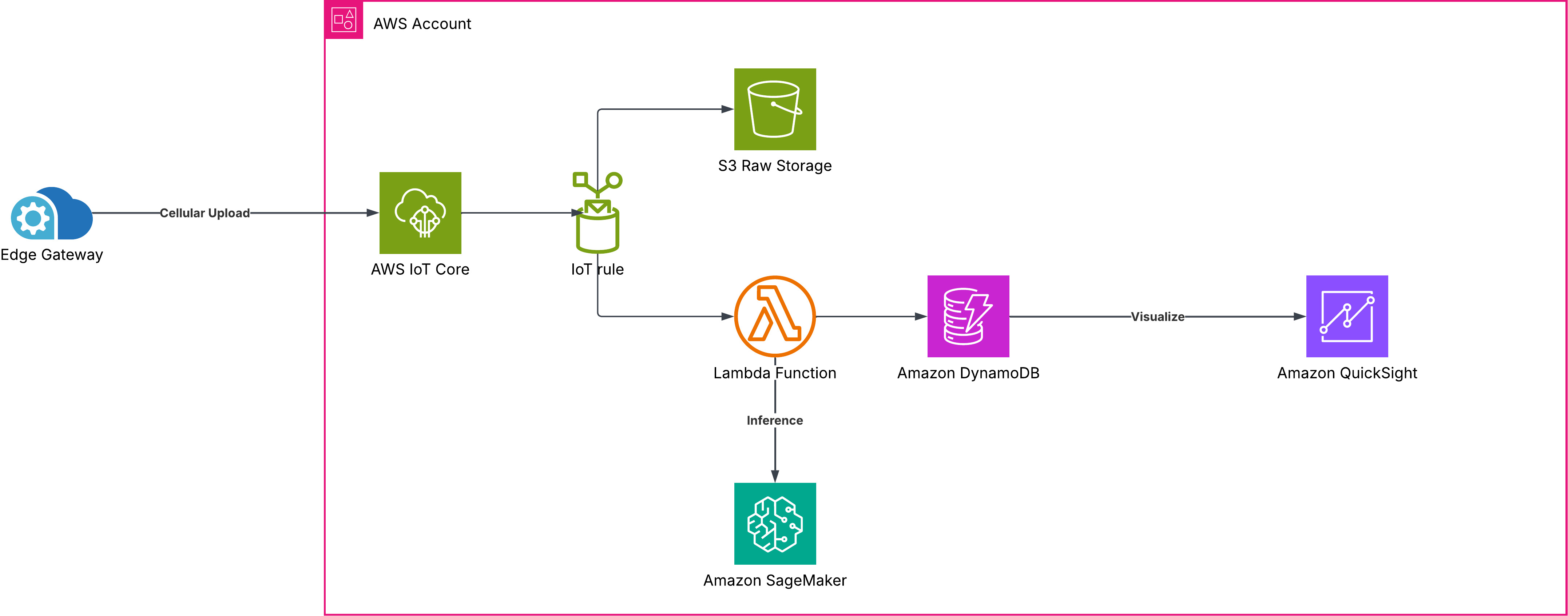
| Line item | Monthly |
|---|---|
| Cellular data (5.2 GB, small-account pooled plan) | ~$75 |
| AWS IoT Core messaging, batched 60 readings/message | ~$1.30 |
| S3 storage | ~$0.12 |
| SageMaker real-time endpoint (small, always-on) | ~$85 |
| Total | ~$160/month |
Two observations. First, batching has a large effect on the IoT Core line: sending each reading as an individual MQTT message costs $25.92/month, while batching one minute of readings into a single 12 KB message costs $1.30 for the same data. Second, the AWS charges are small relative to the carrier bill and the inference endpoint.
Upfront cost is effectively zero.
Edge Configuration
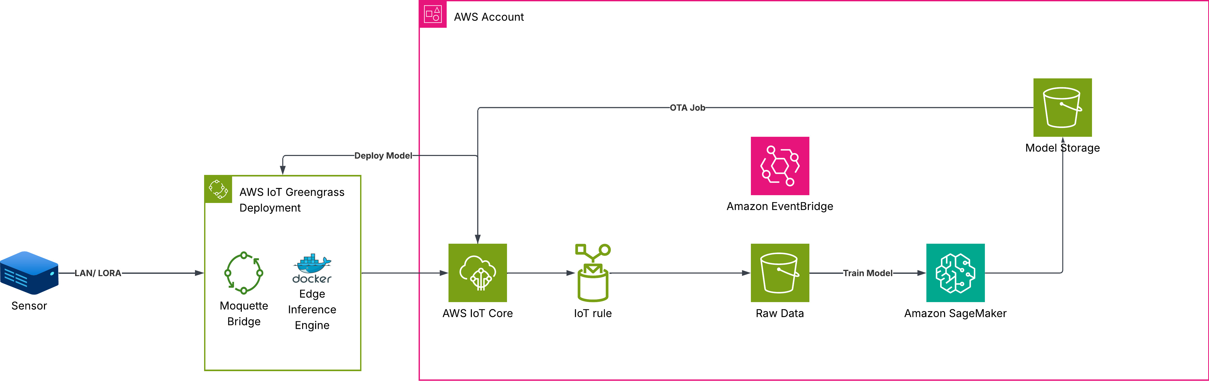
| Line item | Cost |
|---|---|
| Industrial gateway (one per site) | $700 one-time |
| Greengrass Core | $0.16/month |
| Cellular data (~86 MB of summaries and events) | ~$3/month |
| AWS IoT Core messaging | ~$0.09/month |
| Recurring total | ~$5/month |
Sensors connect to the gateway over the local network or LoRa at no incremental cost. The gateway runs the model locally, transmits a compact summary every five minutes, and sends a full payload when an anomaly is detected.
Recurring savings are approximately $155/month, which pays back the gateway in 4.5 months. That figure omits the largest cost.
Implementation Cost
Building this to production standard — cross-compiling the model for ARM, packaging Greengrass components, implementing OTA deployment with rollback, adding local store-and-forward buffering, and instrumenting the device sufficiently to diagnose problems remotely — is realistically 60–120 engineering hours. At a blended $150/hour, approximately $12,000.
($700 + $12,000) ÷ $155/month = 82 months to payback
That exceeds the service life of the gateway. At ten sensors, the cloud configuration is the correct choice on cost grounds.
Scenario Two: 500 Devices Across 50 Sites
The same sensors and duty cycle, distributed across fifty buildings.
Recurring savings scale linearly: $15.50 per device per month × 500 = $7,750/month.
Upfront costs do not scale the same way:
- Hardware: 50 gateways × $700 = $35,000, scaling with sites rather than sensors
- Engineering: the same core work plus fleet operations — staged rollouts, canary groups, rollback tooling — approximately $20,000
- Total upfront: $55,000
$55,000 ÷ $7,750/month = 7.1 months to payback
At this scale the edge configuration is clearly justified.
Locating the Crossover
Engineering cost is fixed; savings are per-device. That yields a simple model:
N_breakeven = FixedEngineering ÷ (MonthlySavingPerDevice × HorizonMonths − HardwarePerDevice)
Using the figures above — $20,000 fixed, $15.50 per device per month saved, a 36-month horizon, and $70 per device in amortized hardware (one $700 gateway per ten sensors):
558N > 20,000 + 70N → N ≈ 41 devices
Approximately forty devices is where edge inference begins to pay for itself. On a 24-month horizon the figure is closer to sixty-six.
Device count, however, is not the controlling variable. The calculation depends on $15.50 per device per month of avoided bandwidth, and that figure is a function of bytes per device rather than device count:
- A temperature sensor reporting every five minutes generates roughly 0.5 MB/month. Per-device savings are a few cents, and there is no device count at which edge inference recovers its implementation cost.
- A single 1080p camera streaming continuously generates 300–500 GB/month and justifies an edge deployment on its own, at N = 1.
Edge inference is best understood as a bandwidth trade, with a threshold set by data rate that device count then multiplies. The first calculation to run is bytes per device per month. Below a few hundred megabytes, the cloud configuration will generally win regardless of fleet size.
Requirements That Override the Cost Analysis
Four cases where the calculation above does not determine the answer:
- Control loops. If inference results actuate equipment — shutting down a compressor, stopping a conveyor, triggering a safety interlock — a round trip that is 200 ms under normal conditions and several seconds during a network event is not viable. Edge inference is required at any device count.
- Unreliable connectivity. Mine sites, rural pump stations, agricultural equipment, and mobile assets crossing coverage gaps all need to continue operating while offline. Decision logic runs locally; the cloud handles reporting and retraining.
- Data transmission constraints. Cameras in patient areas, footage capturing third-party property, and similar cases may carry regulatory or contractual limits on what can be transmitted. Running inference locally and sending only derived metadata is often what makes the architecture viable.
- Video and high-rate vibration. Anything sampling above roughly 1 kHz or producing image frames has already crossed the data-rate threshold, and the calculation is unnecessary.
A Cloud-First, Edge-Ready Approach
The framing above is binary; production architectures usually are not. For most teams starting out, the practical approach is to build in the cloud while keeping an edge migration a deployment change rather than a rewrite:
- Implement preprocessing once and run it in both environments. The transformation from raw readings to model features should be a single versioned Python package. Whether it executes in a Lambda function or a Greengrass component then becomes a packaging question.
- Define an explicit feature contract. The model consumes a documented feature vector; where that vector is computed sits behind a stable interface.
- Include store-and-forward buffering at the edge from the start, even in a cloud-first build. It is inexpensive to add early, difficult to retrofit, and protects data quality when connectivity is intermittent.
- Track bytes per device per month as a monitored metric. This is the value that triggers a migration decision, and it is frequently not measured until it appears on an invoice.
Built this way, migrating from cloud to edge is a few weeks of packaging and rollout work — roughly $6,000 rather than $20,000. Applying that to the breakeven formula moves the crossover from approximately forty devices to approximately thirteen.
The fixed engineering cost is both the largest term in the calculation and the one most within your control. Keeping it low means the edge-versus-cloud decision does not have to be made before the project starts.
Fastwater Cloud builds IoT and AI systems on AWS for small and medium sized businesses. If you are evaluating this decision, or reviewing connectivity costs on an existing deployment, we are glad to work through the numbers with you.